Hardy - Cross method - Head balance method for flow loops

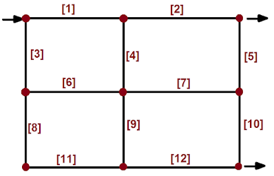
 The main idea behind the Hardy-Cross method is to force a head loss $h_L$ balance among all pipes which are part of a flow loop. Without the $h_L$ balance flow rates, which are usually the unknown, cannot be determined. There are other methods but this is the most familiar.

This methodology, as you may already know, is based on the general equation for mechanical energy balance, so that every loop in the above network must be decomposed in smaller parts, which are in fact the pipe sections.

Note: A loop is a circuit of flow. In other words, a loop is formed by interconnected pipe sections through wich the fluid may travel in a given direction. For example, pipe sections [1], [4], [6] and [3] form a loop.

Then, for any of the 12 pipe sections in the network above has a particular head loss defined as follows,

$h_L^{(n)}=f_F^{(n)}\frac{L_n}{D_n}\frac{v_n^2}{2g}$        Eq. (1)

or as,

$h_L^{(n)}=f_F^{(n)}\frac{L_n}{D_n}\frac{8Q_n^2}{\pi^2 D_n^4 g}$        Eq. (2)

where $n$  indicates any of the pipe sections in a loop ([1], [4], [6] or [3], for example). Also $n$ was written in parenthesis $(n)$ to avoid confusion with powers. Several textbooks authors like to write Eq. (2) as,

$h_L^{(n)}=K_nQ_n^2$        Eq. (3)

where $K$ is defined as,

$K_n=f_F^{(n)}\frac{L_n}{D_n}\frac{8}{\pi^2 D_n^4 g}$        Eq. (4)

Following, with Hardy-Cross technique a head losses balance forming a loop is made. In a very general form, this would look like,

$\sum_{n=1}^{n=m}h_L^{(n)}=0$        Eq. (5)

where $m$ is the total number of pipes forming the loop. For example, for each loop in the network above, $m=4$.

Now, as the $h_L$ balance is not zero per se the way to forcing it to be zero is by small adjustments on the flow rates. Substitution of Eq. (3) into Eq. (5) gives,

$\sum_{n=1}^{n=m}K_n Q_n^2=0$        Eq. (6)

and if you add a small flow rate correction $\Delta Q$ to each pipe section, Eq. (6) becomes,

$\sum_{n=1}^{n=m} K_n \left( Q_n+\Delta Q \right)^2=0$        Eq. (7)

 Expansion of Eq. (7) produces,

$\sum_{n=1}^{n=m} K_n \left[ Q_n^2+2Q_n\Delta Q+\left( \Delta Q \right)^2 \right] =0$        Eq. (8)

Since the flow corrections $\Delta Q$ are small (smaller than 1), then powers of it can be neglected. Thus, Eq. (8) can is reduced to,

$\sum_{n=1}^{n=m} K_n \left[ Q_n^2 + 2Q_n \Delta Q \right] =0$        Eq. (9)

and since $\Delta Q$ is not particular to any pipe section (do not depend of $n$) a further simplification is possible,

$\sum_{n=1}^{n=m} K_n Q_n^2 + 2\Delta Q \sum_{n=1}^{n=m} K_n Q_n=0$        Eq. (10)

Next, the flow rate correction $\Delta Q$ can be easily isolated form Eq. (10) to be,

$\Delta Q =- \frac{\sum_{n=1}^{n=m} K_n Q_n^2 }{2\sum_{n=1}^{n=m} K_n Q_n}$        Eq. (11)

Equation (11) can also be written in terms of $h_L$ to ease calculations,

$\Delta Q = - \frac{\sum_{n=1}^{n=m} h_L^{(n)}}{2\sum_{n=1}^{n=m} h_L^{(n)}/Q_n}$        Eq. (12)

Finally, the correction $\Delta Q$ given in Eq. (12) must be applied iteratively to each loop so that with each iteration $\Delta Q$ decreases assuring that the $h_L$ balance is approaching to zero.

At this point, the mass balance has not been mentioned but this is part of the weaknesses of the method.

Any question? Write in the comments and I shall try to help.

=========

Ildebrando.