Minimum square method

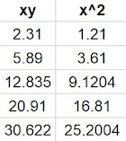
 Example for fitting data to a straight line

The minimum, or least, square method is a reliable numerical method for fitting data to empirical equations. In this case, the simple straight line with familiar equation is,

$y=mx+b$        Eq. (01)

is the one to be used with the slope $m$ and intercept $b$ as the free parameters. In other words, $m$ and $b$ should be estimated from the given data so that the straight line adjust itself, as much as possible, to the data points.

Important note: If you are new to fitting data any given equation you should be aware that the set of data points, if plotted, should beave linearly. This is, the plotted data points should look as if these wer along a straight line. 

The sample data

Let us consider the following set of (x,y) data points as shown in the table below,

Table 1. Sample data for fitting to a straight line

Basic equations for the minimum (or leasts) square method for fitting to a straight line

If experimental data, as thos shown in Table 1, were to be represented by a straight line given in general form by Eq. (01), then the slope $m$ and intercept $b$ can be estimated by the following formulas,

$m=\dfrac{N\sum (xy)-\sum (x) \sum (y)}{N\sum(x^2) - \left(\sum x\right)^2}$        Eq. (02)

$b=\dfrac{\sum (y) - m\sum (x)}{N}$        Eq. (03)

In Eqs. (02,03) the symbol $\sum$ means summatory. It is expected to have several lines of data so that these have to be summed up as indicated by the formulas.

As may notice, the main difficulty comes from the amount of data. If you were to handle hundreds of points the calculations bay hand and calculator could take very long so that the use of a worksheet is necessary.

Example minimum (or leasts) square method calculations

From Eqs. (02,03) it can be easily seen that a numer of summations are needed,

$\sum (xy), \sum (x), \sum (y),\sum(x^2) $

Then organizing the calculations in tables we can quickly arrived to,

Table 2. Calculations of products row by row

Fig. 1 Plot of data points in Table 1. Notice that the data looks very close to what you could call a straight line.

And from the above calculations we can easily evaluate the summations as,

$\sum (x)=15.14$

$\sum (y)=20.65$

$\sum (xy)=72.567$

$\sum(x^2)=55.9508$

and

$\left(\sum x\right)^2=229.2196$

With the above results calculation of $m$ and $b$ is not difficult. Substitution of the above results into Eqs. (02,03) gives,

$m=0.9932$

$b=1.1223$

Finally, the equation of the straight line that better fits or represents the experimental data in Table 1 is,

$y=0.9932x+1.1223$        Eq. (04)

Here is a Google Sheets worksheet that may help you to understand and perform your own calculations. Make a copy of the file so that you can modify it at pleasure,

Minimum square method linear fitting example

Any question? Write in the comments and I shall try to help.

Other stuff of interest

• Some basic concepts on thermodynamics
• Who was Clausius?
• Units conversion
• LE 04 - Latch contact with encapsulated relay for turning on/off an AC bulb light
• About PID controllers
• Ways to control a process
• About pilot lights
• Solving the Colebrook equation

==========
Ildebrando.