ChemEng stuff followers

Showing posts with label pressure. Show all posts

Sunday, August 17, 2025

A case of conversion - From $lb_m$ to $gpm$

 Imperial units prove to be somtimes hard to use. Here the case of conversion from mass to volumetric flowrate is presented.

As one may imagine a physical property of the fluid is required: the density $\rho$. This can be written as,

$\dot{Q}= Q\, \rho$        Eq. (01)

where $\dot{Q}$ is the mass flow rate, in $lb_m/hr$ for example, and $Q$ is the volumetric flow rate, in $gpm$, for example.

Let us now consider the case of $40,000.00\, lb_m/hr$ flowing liquid water at $190\,^\circ \, C$. In this case, its density would be $\rho=54.70\,lb_m/ft^3$.

Using Eq. (01), it follows,


$Q=\dfrac{\dot{Q}}{\rho}=\dfrac{40,000.00\, lb_m/hr}{54.70\, lb_m/ft^3}$
$Q=924.56\,ft^3/hr=115.27\,gpm$

which is the desired conversion. If you were working with steam, working pressure must be considered to get the proper fluid density.

Sunday, August 10, 2025

Commercial steel pipe Schedule 80 data

 You should be familiar with the data provided in the Appendix B of Flow of fluids through valves, fittings and pipes, for commercial steel pipes with schedule 40 for the flow of water and air.


Several questions always arise: what is the data for schedule 80 commercial steel pipe? what are the data for other pipes (PVC, copper, etc.)? This  data is available on the internet and you should search for it. However, this post is devoted to provide the data for commercial steel pipe schedule 80 and to serve as proof that this information is provided by the manufacturers.

Here, two files are provided:

Make a comparison with the data provided in the reference mentioned early. These files data are for water too.


Wednesday, March 26, 2025

On the vapor pressure data for different NaCl dilutions at different temperatures

 The data presented in this post were extracted from the International Critical Tables.

As is usual in evaporation operations the boiling temperature elevation (BPE) is a key data for engineering calculations. Then, the vapor pressure for different combinations of solute concentration and temperatures are to be combined with the Duhring approximation (Duhring's lines).

The data was just rewritten from the source previously mentioned.


Vapor pressure, mm Hg
Wt % 0.0 2.5 5.0 7.5 10.0 12.5 15.0 17.5 20.0 22.5 25.0 27.5
t °C
0 4.579 4.5 4.4 4.4 4.3 4.2 4.1 4.0 3.8 3.7 3.5
10 9.21 9.1 8.9 8.8 8.6 8.4 8.2 8.0 7.7 7.4 7.1
20 17.54 17.3 17.0 16.7 16.4 16.1 15.7 15.3 14.8 14.2 13.6
30 31.83 3.4 30.9 30.4 29.8 29.2 28.5 27.7 26.8 25.8 24.7
40 55..34 54.5 53.6 52.7 51.7 50.7 49.5 48.1 46.6 44.9 43.0
50 92.54 91.2 89.7 88.1 86.4 84.7 82.8 80.5 78.1 75.3 72.2
60 149.46 147.2 144.8 142.3 139.7 136.8 133.7 130.0 126.0 121.7 116.8
70 233.79 230.2 226.4 222.4 218.3 213.9 208.9 203.5 197.5 190.7 183.1
80 355.47 350 344 338 332 325 318 309.5 300.5 290.2 278.9 266
90 526 517 509 500 491 481 470 458 445.1 430 414 395
100 760 748 736 723 710 695 680 665 643 622 599 572
110 1075.4 1057 1040 1022 1003 983 961 936 911 881 849 810
B. P., °C 100 100.44 100.9 101.4 101.93 102.51 103.16 103.89 104.72 105.68 106.78 108.12

Thursday, January 9, 2025

Enthalpies in the steam tables

 Enthalpy is a thermodynamic concept that can be hard to get a grip on. Perhaps, the reason is that it appears in several contexts so that understanding of it becomes confusing.

In this post the usage of enthalpy in the context of steam is presented. This is an interesting case since steam services are present in almost every chemical process industry and different daily applications, such as the heating of buildings, for example.

On the other hand, the interpretation of enthalpy, among the professionals of the steam, is as  thermal energy (as simple as that). Why? Because, engineers and technician need something easy to use and measurable rather than something that makes their work harder.

Some parameters used in steam tables

Data in steam table are usually order either by pressure or by temperature. Also there are different two types of steam: saturated and superheated. For simplicity, we will only refer to saturated steam tables.

For reference, consult the ASME Steam tables. Compact edition book.

Fig. 01 Sample steam tables by temperature and pressure. These tables were taken from the ASME Steam Tables. Compact edition book.

The steam tables present data for volume, enthalpy and pressure. In this post, we will focus on volume and enthalpy only.

Volume of liquid and vapor

These parameters, appearing in the columns 3 and 4 in tables of Fig. 01, partly indicate how much liquid water is present in the steam. Unless the steam is completley dry the steam will be a two phase fluid made of: vapor and liquid (in the form of small droplets). As you  can see from the data in tables of Fig. 01, the saturated steam is not dry at all.

This volume is presented as [volume of liquid or vapor]/[unit mass of steam]. In other words, and for the present case, this is the $ft^3$ of liquid or vapor per $lb_m$ of steam. Also, the summation $V_L+V_V$ is also called the specific volume.

The enthalpies

In Fig. 01 only two enthalpies ares shown: $h_L$ and $h_V$. However, a third enthalpy parameter usually appear in this kind of tables: $h_{evap}$. Theses parameters can be referred as,

  • $h_L$ the enthalpy of the liquid phase,
  • $h_V$ the enthalpy of the vapor phase and
  • $h_{evap}$ the enthalpy of evaporation,

all in the same units: $Btu/lb_m$ or $kJ/kg$ (for SI units). In fact,

$h_{evap}=h_V - h_L$

For illustration purposes, let us consider the first row, for steam at $32\,F$, in Table 1 of Fig. 01. Thus, $h_L$ is interpreted as the energy required to increase the temperature of $1\,lb_m$ of water (or $1\,kg$ of water, in SI) from its freezing point to its boiling temperature $32\,F$ for the present case. Notice, that $h_L$ will only make sense if the water remains liquid.

For the same row in Table 1 in Fig. 01, $h_{evap}$ is interpreted as the energy required for the change of phase of $1\,lb_m$ (or $1\,kg$ in SI) of liquid water at its boling temperature into vapor. Notice, that either liquid or vapor are at $32\,F$, the boiling temperature. This amount of energy referred by the steam professionals as the one that can be used for heating purposes since the steam can very quickly transfer it.

Finally, $h_V$ is interpreted as the thermal energy carried by the vapor. This is the energy of the liquid at its boiling temperature plus an added energy so that the fluid can be in vapor phase.

One parameter I have no mentiones is the pressure. All above comments are for constant pressure. If you change the pressure, the values of temperature, volume and enthalpies will also change but the interpretation will be the same.

Any question? Write in the comments and I shall try to help.

Other stuff of interest

Monday, August 28, 2023

Composition variables for mixtures

 When composition of a mixture of several gases is to be considered it can be challenging to use all concepts to represent the right quantities. This is a brief explanation.

About mole $n$ and volume $V$

The number of moles for a pure substance is usually represented by $n$. However, for a mixture with several components the moles of each of these components are to be expressed as follows:

$n_1$, $n_2$, $n_3$,...


where the subscripts 1, 2, 3 indicate the component in the mixture. 


Important note: You should remember that moles are extensive variables which is not recommended for composition calculations purposes. You may go around this difficulty dividing $n$ by an intensive variable, which results in a new intensive variable.


On the other hand, you may also have volumetric concentrations [concentración volumétrica] $\bar{c}$ defined as:

$\bar{c}_i=\dfrac{n_i}{V}$


where $n_i$ stands for the mole of some component and $V$ for the volume of the mixture. When $\bar{c}$ is given in units such as mole/l or mole/dm$^3$ the volumetric concentration is also called molar concentration [molaridad].


Important note: volumetric concentration is recommended for liquid or solid mixtures since these change very little with temperature and pressure. However, the use of $\bar{c}_i$ is not advised for gas mixtures. 


Mole ratio $r_i$ and molal concentration $m_i$

This is another form for referring to composition in terms of moles of components in a mixture. Picking up the moles of component 1 as reference we may define the corresponding ratios $r_i$ for all others as:


$r_i=\dfrac{n_i}{n_1}$


On the hand, molal concentration $m_i$ is in fact a variation of the mass concentration (how it is expressed) of the single component  gas $m$. Remember that the mass $m$ can be defined as:


$m=nM$


where $M$ is the molar mass (molalidad) given in [mole/g]. However, the mass of a component in a gas mixture is defined as:


$m_i=\dfrac{n_i}{n_1M_1}=\dfrac{r_i}{M_1}$


In other words, the mass $m_i$ of a mixture component must be given in terms of the mass and moles of the other components.

Since mole and molality ratios are temperature and poressure independent, these are preferable for any physicochemical calcuation.

Mole fractions $x_i$

These are obtained dividing each of the number of moles ($n_1$, $n_2$,...), of each component, by the total number of moles $n_t$ (of the whole substance) which is defined as:


$n_t=n_1+n_2+n_3+...$


The mole fraction is then expressed as,


$x_i=\dfrac{n_i}{n_t}$


Also, the summation of the mole fractions is always equal to 1:


$x_1+x_2+x_3+...=1$


Important note: The composition of a mixture is determined when all mole fractions are given or can be determined. Since mole fractions are temperature and pressure independent, these are suitable, and possibly the most used, to describe the composition of any mixture.


Any question? Write in the comments and I shall try to help.

Other stuff of interest

Tuesday, July 4, 2023

About the PID controller

 For short, it is an electronic device capable of controlling a process variable such as temperature or pressure, for example.

A little of technical background

The origin of PID controllers is on the well known mathematical expression:

$CO(t) = Bias - K\left[SP-PV(t)\right] - \dfrac{K}{t_i}\int_0^{\tau=t} \left[SP-PV(\tau)\right] \; d\tau - K t_d \dfrac{d}{t}\left[ SP-PV(t) \right]$        Eq. (01)

where $CO(t)$ stands for the controller output, $Bias$ for the situation at which the measured process variable equals the set point, $SP$ for the constant set point, $PV(t)$ for the measurements of the time dependent process variable, $K$ for the controller gain, $t_i$ for the integral time and $t_d$ for the derivative time. Equation (01) deserves a more detrailed explanation but it is leaved for another post.

For now, it should be sufficient to say that $CO$ is in fact a signal that is to be used to modulate the operation the final element of control, say a valve or motor, for example. From the practical point of view, Eq. (01), if applied to any process variables, should be enough to keep a process variable as close as possible to its set point (there are some further details to discuss for this assumption so that this is not always true).

The real PID controller

In practice what you have is a device following the rule established in Eq. (01) along with a number of problems and technical solutions already available in the market. It is not clear for the undergraduate student that in real life control situations you would need for example:

  • measure temperature with a thermocouple, an RTD or a infrared sensor,
  • register the process variable data,
  • create a ramp for the process variable,
  • probably use On/Off instead of PID,
  • control pressure instead of temperature,
  • among other things.
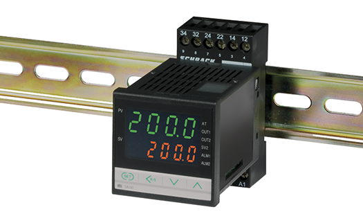
Other details would have to be listed above but the point is that implementation of a PID control requires technical details not available in Eq. (01). Then it should not be strange that a real life PID controller could have different presentations and different prices. Take a look to the following examples:
Fig. 1 PID controllers

Some of the above shown will fit for particular applications and budgets. The features of these controllers examples may differ according to the brand and not all would be classified as PID controllers but as thermostats.

Perhaps, the most common PID controller is related to temperature as the process variables and its operation/installation/usage would be suitable for thermal applications. However, PID control may also be used for other process variables such as pressure or flow rate which would introduce different technical issues.

Fig. 2 Schematics of how to wire a PID controller

Technicalities

Using a PID controller requires more than just knowing Eq. (01) but knowing about sensors and electricity. As shown in Fig. 2, controlling temperature, for example and accoirding to the controller in Fig. 2, requires to choose between two possible sensors: thermocouples and RTD's; and to adjust the electrical supply to alternate current between 110 to 240 V so that the controller could be powered. We may go further since a particular probe for the sensor would be needed!


PID controller installation/selection would also lead to another disjunctive. Panel mounted versus rail DIN installation. At first this is important from the point of view of available space but it intrinsically means plannification before buying a possibly expensive control device.

Fig. 3 Rail DIN installation of a PID controller

There are many other PID controller models available in the market and it would be difficult to mention all of these. The most important conclusion of this post would be need to understand how to translate the physics behind Eq. (01) into the usage of devices in Figs. 1-3 in order to control a process variable.

Theoretical understanding of Eq. (01) is very important but for the practicing engineer technical knowledge must be added.

Any question? Write in the comments and I shall try to help.

==========
Ildebrando.


Saturday, June 3, 2023

Hardy - Cross method - Head balance method for flow loops

 The main idea behind the Hardy-Cross method is to force a head loss $h_L$ balance among all pipes that are part of a flow loop. Without the $h_L$ balance flow rates, which are usually the unknown, they cannot be determined. There are other methods, but this is the most familiar.


This methodology, as you may already know, is based on the general equation for mechanical energy balance, so that every loop in the above network must be decomposed into smaller parts, which are in fact the pipe sections.

Note: A loop is a circuit of flow. In other words, a loop is formed by interconnected pipe sections through which the fluid may travel in a given direction. For example, pipe sections [1], [4], [6], and [3] form a loop.

Then, for any of the 12 pipe sections in the network above, a particular head loss is defined as follows,

$h_L^{(n)}=f_F^{(n)}\frac{L_n}{D_n}\frac{v_n^2}{2g}$        Eq. (1)

or as,

$h_L^{(n)}=f_F^{(n)}\frac{L_n}{D_n}\frac{8Q_n^2}{\pi^2 D_n^4 g}$        Eq. (2)

where $n$  indicates any of the pipe sections in a loop ([1], [4], [6], or [3], for example). Also, $n$ was written in parentheses $(n)$ to avoid confusion with powers. Several textbook authors like to write Eq. (2) as,

$h_L^{(n)}=K_nQ_n^2$        Eq. (3)
where $K$ is defined as,

$K_n=f_F^{(n)}\frac{L_n}{D_n}\frac{8}{\pi^2 D_n^4 g}$        Eq. (4)

Following the Hardy-Cross technique, a head loss balance that forms a loop is created. In a very general form, this would look like,

$\sum_{n=1}^{n=m}h_L^{(n)}=0$        Eq. (5)

where $m$ is the total number of pipes forming the loop. For example, for each loop in the network above, $m=4$.

Now, since the $h_L$ balance is not zero per se, you can force it to be zero by making minor adjustments to the flow rates. Substitution of Eq. (3) into Eq. (5) gives,

$\sum_{n=1}^{n=m}K_n Q_n^2=0$        Eq. (6)

and if you add a minor flow rate correction $\Delta Q$ to each pipe section, Eq. (6) becomes,

$\sum_{n=1}^{n=m} K_n \left( Q_n+\Delta Q \right)^2=0$        Eq. (7)

 Expansion of Eq. (7) produces,

$\sum_{n=1}^{n=m} K_n \left[ Q_n^2+2Q_n\Delta Q+\left( \Delta Q \right)^2 \right] =0$        Eq. (8)

Since the flow corrections $\Delta Q$ are minor (smaller than 1), then powers of it can be neglected. Thus, Eq. (8) can be reduced to,

$\sum_{n=1}^{n=m} K_n \left[ Q_n^2 + 2Q_n \Delta Q \right] =0$        Eq. (9)

and since $\Delta Q$ is not particular to any pipe section (does not depend on $n$), a further simplification is possible,

$\sum_{n=1}^{n=m} K_n Q_n^2 + 2\Delta Q \sum_{n=1}^{n=m} K_n Q_n=0$        Eq. (10)

Next, the flow rate correction $\Delta Q$ can be easily isolated from Eq. (10) to be,

$\Delta Q =- \frac{\sum_{n=1}^{n=m} K_n Q_n^2 }{2\sum_{n=1}^{n=m} K_n Q_n}$        Eq. (11)

Equation (11) can also be written in terms of $h_L$ to ease calculations,

$\Delta Q = - \frac{\sum_{n=1}^{n=m} h_L^{(n)}}{2\sum_{n=1}^{n=m} h_L^{(n)}/Q_n}$        Eq. (12)

Finally, the correction $\Delta Q$ given in Eq. (12) must be applied iteratively to each loop so that with each iteration $\Delta Q$ decreases, assuring that the $h_L$ balance is approaching zero.

At this point, the mass balance has not been mentioned, but this is a weakness of the method.

Any questions? Write in the comments, and I shall try to help.

=========
Ildebrando.
Friday, May 26, 2023

Some thoughts about pipe mechanical features

Perhaps what follows may be obvious for experienced professionals but this may  not be true for the engineering student. Hopefully, this will be useful.

  1. Pressure and flow rate are related. This is, theoretically, stated by the energy and Bernoulli equation. Besides, this is also tru in practice. Increment and decrement of flow rate are related to changes in pressure.
  2. Flow rate increases with diameter; but also with pressure. If you wish to increase the flow rate two options are available: a) you may choose a larger pipe diameter or b) you may increase pressure. If you choose to increase pressure you must know that this cannot be changed arbitrarily and without control.
  3. The minimum flow rate is key. The reason is simple. When a pipe system is designed, it is so to operate under steady conditions at the lowest possible cost (without sacrifyce of safety, service life, etc.). Otherwise, you will be wasting money.
  4. Different pipe sizes may tranport the same flow rate. This is that, commercial steel pipes with ND 1", 1.5" and 2" may transport the same volume of fluid per minute for certain conditions. In other words, you could, theoretically, estimate the internal pipe diameter but in practice different real pipes may be available to transport the very same flow rate at a lower cost.
  5. Pipes may fail. This is that, in contrast with the classroom situations, the engineer should pay attention to the maximum pressure that the pipe may work at (before increasing the flow rate). Even steel pipes may burst or crack at overpressure conditions creating a real chaos.
  6. Be aware of phase changes. Phase changes may induce vacuum in the pipe exerting enormous local mechanical stresses in the pipe and creating risk for the structure. This is not apparent; but accessories like safety valves could be very useful in some cases.
Any question? Write in the comments and I shall try to help.

=========
Ildebrando

A general comment on pipes

The flow of a fluid through a pipe, in several bachelor courses, is studied merely as a theoretical topic. However, in several ocasions instructors tend to use a textbook where flowrate or pressure loss or pipe diameter are unknown and then estimated by means of the energy or Bernoulli equation.


Many textbooks show this. Take for example the following two popular sources:


A more realistic point of view

It comes out that estimation of flow rate or pressure loss or pipe diameter must be complemented with real pipe data that could possibly be installed. In my opinion, these kind of situations must be treated as a design problem. Otherwise, learning is reduced (I think).


In my opinion, it is important that whoever is taking a regular fluid mechanics course should know that there is pipe data indicating its mechanical features. For short, who performs hydraulic calculations should consider the following:


  • nature of the working fluid, where densisty, viscosity, volumetric expansion coefficient, consensation temperature and material compatibility, for example;
  • maximum and minimum flow rate, at which the pipe could work,
  • maximum and minimum pressure expected to be used to move the fluid through the pipe, and
  • maximum and minimum temperature that the fluid will have while being transported.
The previous statements are important because no mater the results of the theoretical calculations, in the end a real pipe satisfying the following factors:

  • safety,
  • life of service y
  • available money, for example
must be selected.

=========
Ildebrando

Most popular posts