In this post, the demonstration of the Hardy-Cross method is extended for its implementation. There are ideas to be introduced and technical difficulties to be solved along the way.
1 Things to set before Hardy-Cross method calculations
1 Things to set before Hardy-Cross calculations
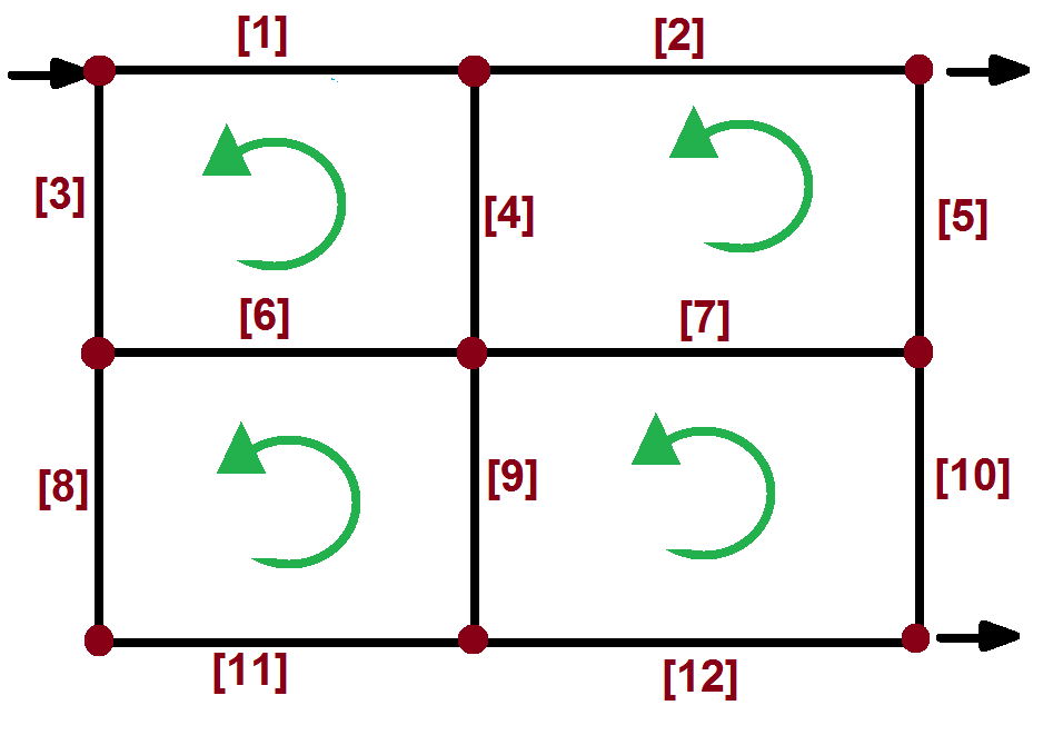
Let us consider a simple network as shown below,
 |
| Fig. 01 A simple 4-loop pipe network. |
Consider that you have the following data about this network:
- pipe material,
- nominal pipe size,
- pipe length,
- discharge flow rate at the two points and
- elevations or angle inclination of each pipe section.
Let us introduce then, two interesting concepts or ideas:
1.1 A node
This refers to a location in the pipe network where the fluid exits the network (and there can be several) or it may enter the network (of which several may exist too). In a node, pipe sections from different loops can also join. On the other hand, a bend or change in direction of a pipe section is not a node. A node implies branching the pipe.
 |
| Fig. 02 Nodes identification in a network. |
Since a pipe network may have several nodes, these are also labeled or numbered in a convenient way to ease calculations.
1.2 Flow and head loss balance direction
Flow direction is key, but its determination in a flow loop can be confusing. In most textbooks, flow direction is usually provided. However, in real-life applications, flow directions need to be set by the engineer treating the situation.
There are two types of directions in a network:
- loop head loss balance direction, which can be either clockwise or counterclockwise. No matter the choice you make, all loops must have the same balance direction and
- pipe section flow direction, which refers to just a pipe section as part of a loop.
The following instructions, based on experience and the physics of the network, can be used to determine flow and head loss directions.
Step 1
 |
| Fig. 03 Setting of flow direction (see blue arrows) in the pipes bifurcating from the inlet. |
Step 2
Flow in pipes converging at outlets may have a behavior similar to that presented in Step 1. The fluid would travel in the direction of the outlet.
 |
| Fig. 03 Setting of flow direction (see blue arrows) in the pipes converging to the outlets. |
Step 3
Use your common sense to determine the missing flow directions (as much as you can). For example, the flow in pipe [7] goes from left to right. At this point, some flow directions have been determined using our experience, but the remaining unknown flow directions require a little more effort.
Step 4
Make use of available pipe data to prioritize a given flow direction. For example, check for the internal or nominal diameters of pipe sections with unknown flow direction. You would expect the flow traveling from a pipe with a large diameter to another one with a smaller diameter.
Another idea you can use is: the farther a pipe section is from an inlet, the smaller its diameter.
Finally, you must also consider elevations at each node. Remember that there is also a hydraulic load to take into account. Make use of the background you have.
Step 5
If you have run out of physical and reliable experience arguments to set the flow directions, all you can do is guess. However, do not worry too much about this, as when you solve for the flow rates, some changes could be driven by the numerical results.
The head balance direction
The head balance is performed according to a prescribed direction. As mentioned earlier, you can set this direction freely. For example, you can choose that head losses in a pipe in which the flow goes from left to right are taken positive, while the head loss in another pipe where the flow is from right to left is negative.
 |
| Fig. 04 Direction set for the head balance calculations. |
You may also consider the other way: clockwise direction. Remember that the only condition to satisfy is that the same direction should be applied for all loops. As you can see, these signs for $h_L$'s give you the balance leading to the equations to be solved.
As an example of a head balance, consider the following two loops from Fig. 04,
 |
| Fig. 05 Sample loops for head loss balance. |
where some flow directions were arbitrarily set. For loop 2, the head loss balance equation would be,
Notice that pipe [7] is shared between the two loops, but the head loss sign changes from one loop to the other. This is, in one loop $h_L^{(7)}$ is taken positive but in the other it is negative.
The mass balance
On the one hand, you already have a head loss balance, but a mass balance can also be obtained. There are several equations for the mass balance, but two categories can be distinguished:
- A global mass balance based on inlets to and outlets from the network, and
- A mass balance at each node. Notice that, if the node is spurious, such as the bent producing pipes [8] and [11], a mass balance can still be done, but its equation gives no helpful information. In other words, you may omit that equation.
What is the usefulness of the mass balance? It helps you to give a guess for the numerical solution to be performed on the equations of the head balance. It also allows for a check on your calculations.
 |
| Fig. 06 A sketch showing how to perform a mass balance at a given node. |
As an example, take the mass balance at the node presented in Fig. 06. Mathematically, it could be written as,
Important note: the mass balance can not be used to solve for the unknown flow rates since equations are missing. The mass balance is not used in the numerical calculation of the unknown flow rates from the head balance, so that the results output by the Hardy-Cross method may sometimes not satisfy the mass balance. You should be aware of this.
2 How to automate calculations in a spreadsheet
Once you have the equations of the problem based on the head loss balance, you can solve it numerically by an iterative procedure. It should be true that the number of equations equals the number of unknowns. Since this method is to be implemented in a spreadsheet, the friction factor must be estimated from a mathematical formula rather than from a graphical method.
Several tables shall be needed. One should be devoted to concentrating all your results. For example, if you are estimating flow rates, it could look as follows,
 |
| Fig. 06 Sample table for registering flow rate results. |
Another table should be devoted to gathering fluid properties and some other parameter numerical values that do not fit in other tables. Here is a sample,
 |
| Fig. 07 Sample table for fluid properties. Be aware of the system units. |
A third table should contain pipe data, such as geometrical features and the like.
 |
| Fig. 08 Sample table for pipe data. Be aware of the system units. |
Also, another table for node data should be needed. In some textbooks, the network has all nodes at the same elevation, but in real life, this is not the case. The relevant information could be gathered as follows,
 |
| Fig. 09 Sample table for node data. |
As you can see, tables in Figs. 06-08 keep some order on the different types of data. Also, notice that all information in the sample tables in Figs. 07-08 is constant, so it does not need to be repeated in the subsequent tables for calculations.
For each iteration performed, a set of tables or a single table encompassing all loop calculations shall be needed. Here, we consider the second option. These tables for each iteration are to be connected among themselves, to the data for pipe and fluid properties, and to the results.
Since the guesses used for iteration #2 are the results of iteration #1, and so on. This table can be as follows,
 |
| Fig. 09 Sample table for iteration #1 calculations. |
 |
| Fig. 10 Sample table for iteration #2 calculations. |
Since every pipe network can have significant differences from other networks, each spreadsheet needs to be prepared or adapted carefully. However, this organization may help identify potential errors in formula programming or similar tasks.
Finally, since changing flow rates modifies the head losses, then pressures at each node and hydraulic load $HGL$ are also changed. In most cases, neither pressure nor $HGL$ is known, so these must be calculated at the end. These results can be gathered in a table as follows,
 |
| Fig. 11 Sample table to collect results on each node. |
Perhaps a better way of understanding the Hardy-Cross method is by solving an example.
This is the end of the post. I hope you find it useful.
Other stuff of interest
- LE01 - AC and DC voltage measurement and continuity test
- LE 02 - Start and stop push button installation 24V DC
- LE 03 - Turn on/off an 24V DC pilot light with a push button
- LE 04 - Latch contact with encapsulated relay for turning on/off an AC bulb light
- LE 05 - Emergency stop button installation
- About PID controllers
- Ways to control a process
- About pilot lights
- Solving the Colebrook equation
- Example #01: single stage chemical evaporator
- Example #02: single stage process plant evaporator
- Example #03: single stage chemical evaporator
- Example #04: triple effect chemical evaporator
- Gas absorption - General comments
- Equilibrium diagrams from gas component solubility data
- Distillation - General comments
- The Hardy-Cross method demonstration
==========
Ildebrando.

No comments:
Post a Comment